Intro
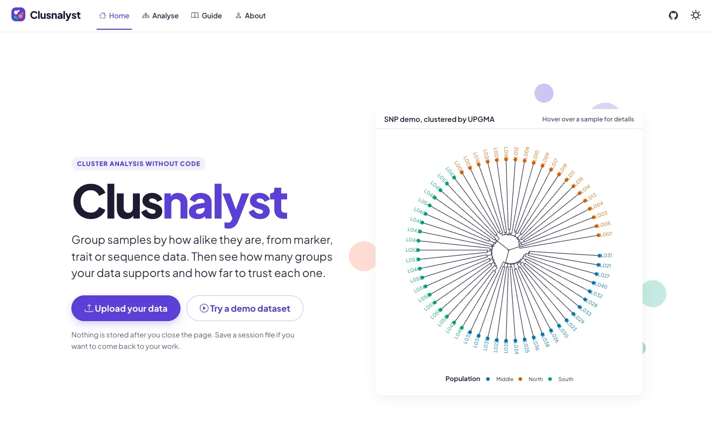
Clusnalyst groups samples by how alike they are, from band scores, SNP genotypes, a sheet of measured traits or a FASTA file. Along with the tree you get bootstrap support for each branch and an estimate of how many groups the data holds. At the end there’s a report to download, plus an R script that repeats the whole analysis.
You can try it in the browser without installing anything.
Where it started
Clusnalyst was our final-year project at KNUST in 2022, built alongside Linkmapper by the same team, which I led. We wrote it to help with teaching systematics. It read 0/1 band scores and letter SNP genotypes, drew a dendrogram and ran silhouette and bootstrap checks. The whole thing was one Shiny file.
What was wrong with it
Four years later I read the old code again and found four bugs that changed results. The options labelled single and complete linkage both ran Ward’s method. The bootstrap resampled columns of the distance matrix instead of the markers, so its support values weren’t valid. Every session shared the same global variables, so two people on the hosted app at once could overwrite each other’s data. And telling it a FASTA file was already aligned made it crash.
Each of those now has a test in the package.
How it works now
- Load a table, VCF, HapMap or FASTA file. The app works out the data type and whether markers are in rows or columns. A second table can add population, origin or coordinates for each sample.
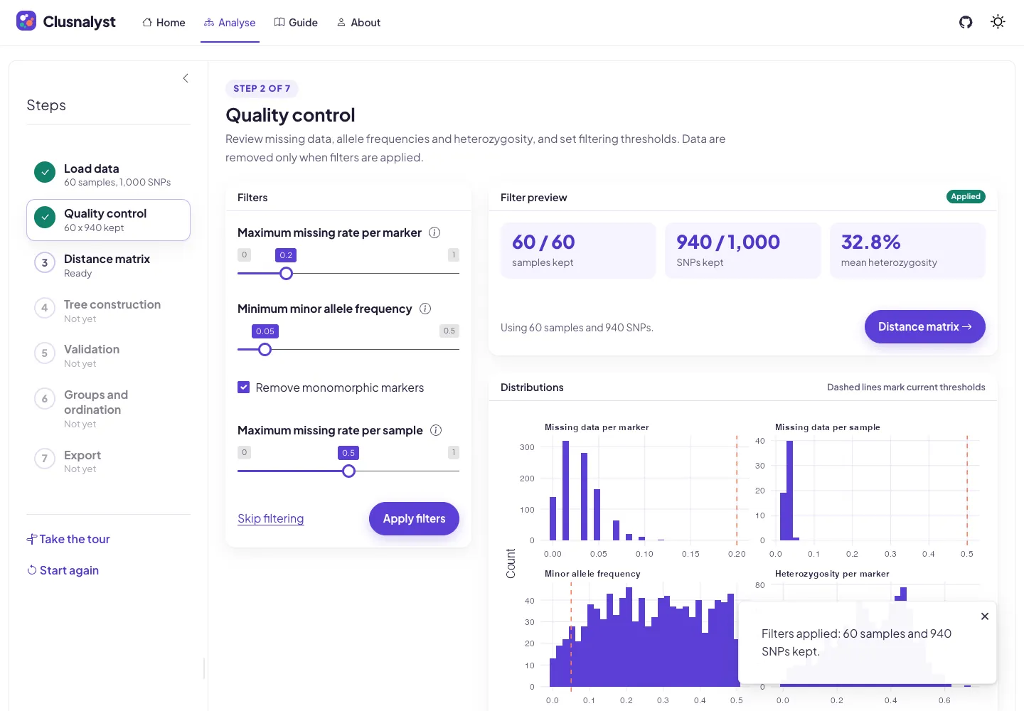
- Check quality: missing data, minor allele frequency and heterozygosity, with filters. Unaligned sequences are aligned with ClustalOmega, ClustalW or MUSCLE.
- Pick a distance. The default depends on the data: Jaccard for bands, allele sharing for SNPs, Gower when some traits are categories, Kimura’s model for DNA.
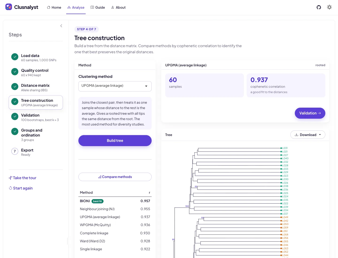
- Build the tree. A table ranks seven methods by cophenetic correlation, so you can see which one keeps your distances best.
- Check it, with bootstrap support from resampled markers, the number of groups by silhouette width and the gap statistic, and a Mantel test against geography or a second matrix.
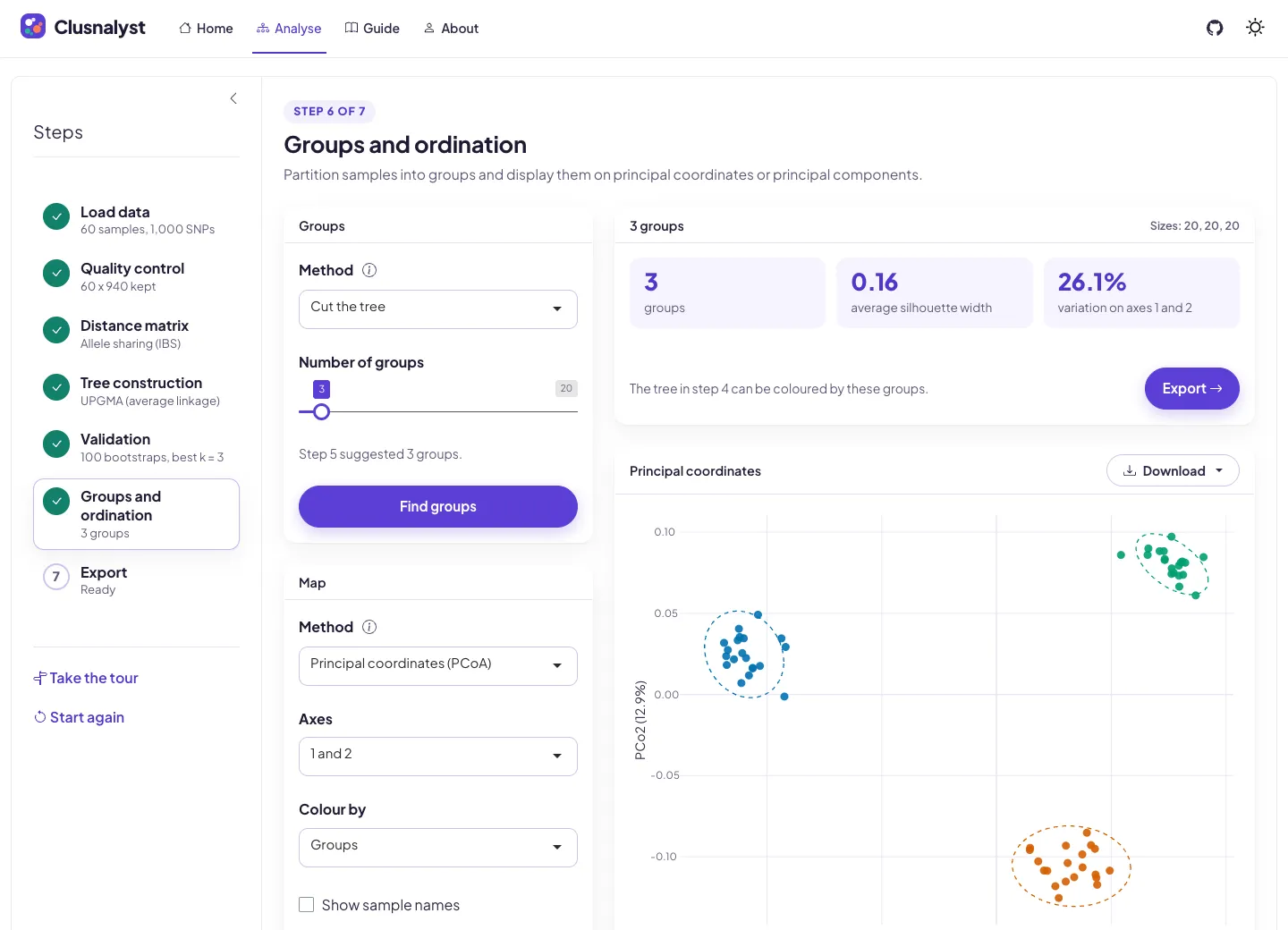
- Split the samples into groups and see them on a PCoA or PCA plot.
- Download a report, the R script and a session file you can open again later.
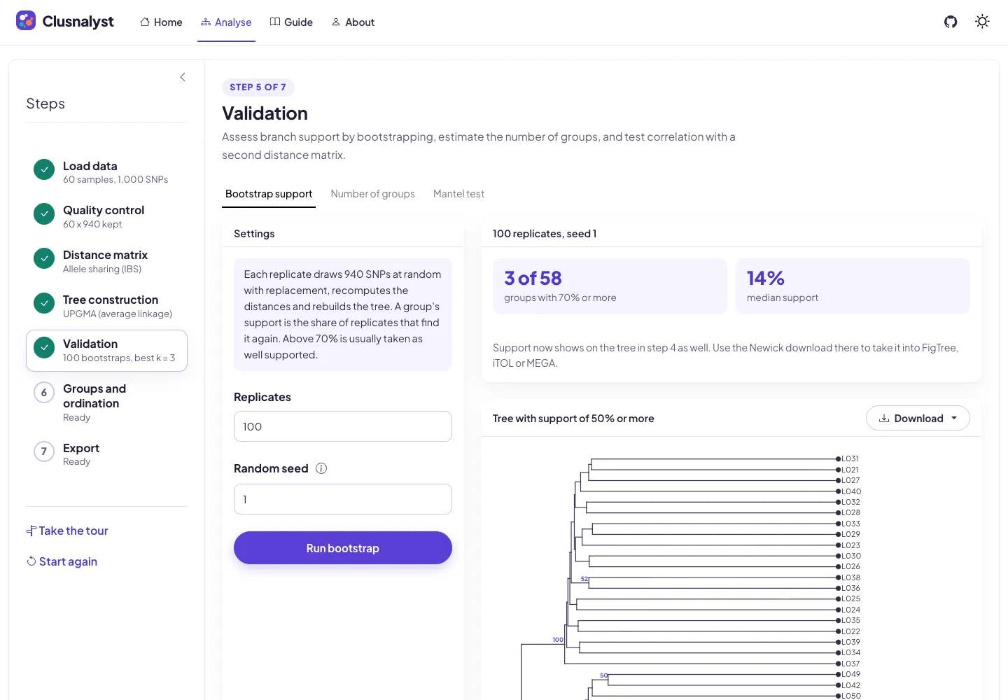
The demo data is simulated: 60 lines from three populations, 1,000 SNPs. Both the gap statistic and the silhouette pick three groups. On the PCoA plot the populations sit in separate corners. The average silhouette width is only 0.16, though, which the usual rule of thumb calls no structure at all. Individual genotypes differ at so many markers that this happens even when groups are real, so the app prints a short note under the number explaining it.
Run it yourself
The hosted copy takes files up to 30 MB and up to 1,000 bootstrap replicates. Installed locally there are no limits:
install.packages("clusnalyst", repos = c("https://ebenogoe.r-universe.dev", "https://cloud.r-project.org"))
clusnalyst::run_app()
Every step is also an exported function, so the analysis can be scripted. The R script the app writes uses the same functions.
What’s next
SSR data with more than two alleles per locus isn’t handled yet, so that comes first. I’d also like the bootstrap to run in the background on the hosted app, so a long run doesn’t hold up the page.