Intro
After FounderForge I wanted the same kind of guided app for getting a good chart out of a spreadsheet, a job far more people have. ggplot2 makes very good charts, but you have to write R to get them. ggWizard puts a step-by-step wizard in front of it.
You bring a CSV or Excel file, check the data, choose a chart, style it and save it. Along with the chart you get the ggplot2 code that draws it and a log of what you did. It’s built the same way as FounderForge, as a golem app inside an R package, so the two share their structure, down to how the files are named.

Bring a spreadsheet
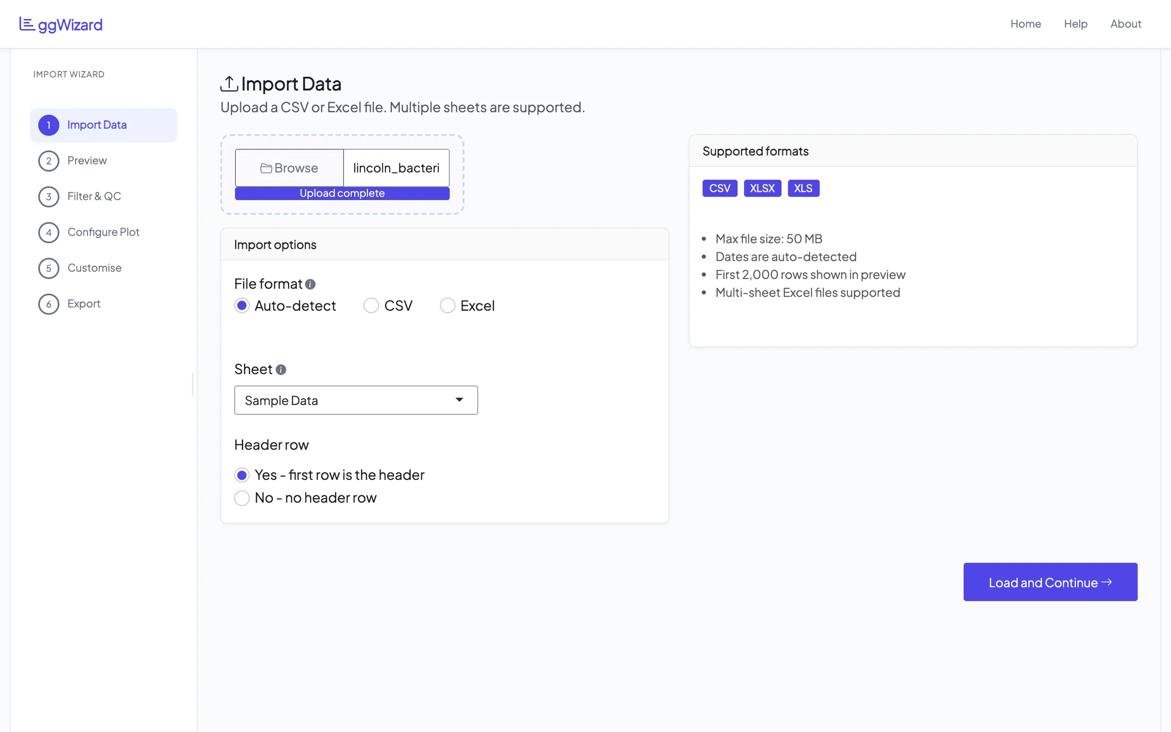
ggWizard reads CSV, XLSX and XLS. If an Excel file has more than one sheet, it lists them and you pick one. It also works out what each column holds, whether numbers, dates, categories, text or yes and no values, because that decides which charts make sense later.
There’s a sample workbook inside the package to try it with. It holds simulated bacteria monitoring data from eight sites around Lincoln, Nebraska, with 268 sampling events and 18 variables. Every screenshot here uses it.
What’s in the file
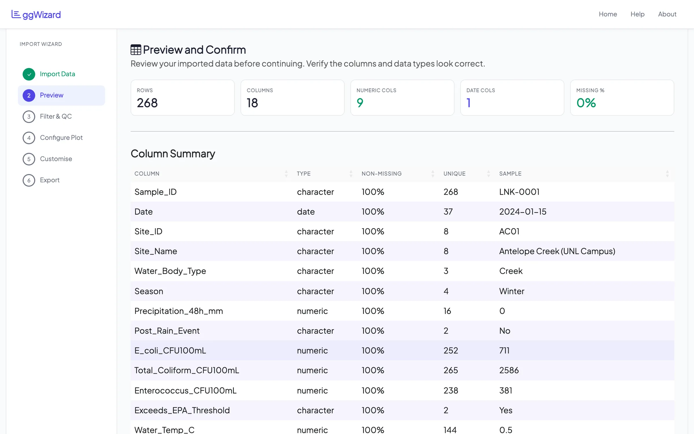
Step two is a summary before you plot anything: rows, columns, how many are numeric or dates and how much is missing. Below it is a table of every column with its type, how complete it is, how many distinct values it has and an example value.
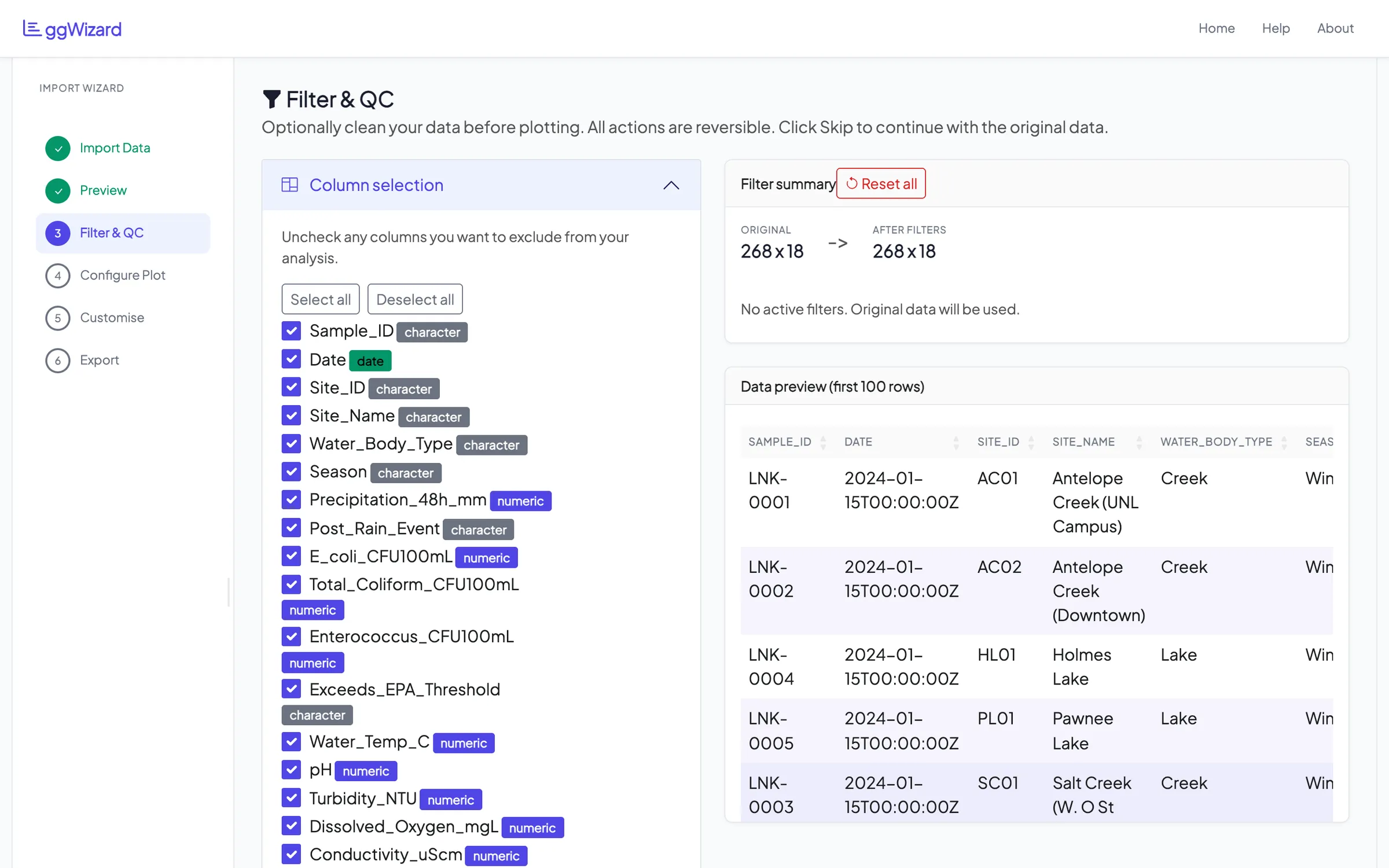
Step three is optional cleaning. You can drop columns you don’t need and flag outliers by Z-score in the columns you pick. There’s a replicate check too, where you choose a grouping column and a measurement. It works out the coefficient of variation within each group and flags the groups above your threshold. Whatever you remove, it shows the size before and after, lets you download the cleaned file and has a reset button.
Pick a chart
There are eight kinds of chart: bar, line, time series, scatter, histogram, box, violin and area. You choose one and map columns to the x and y axes, with colour and separate panels as options. The preview redraws as you change things.
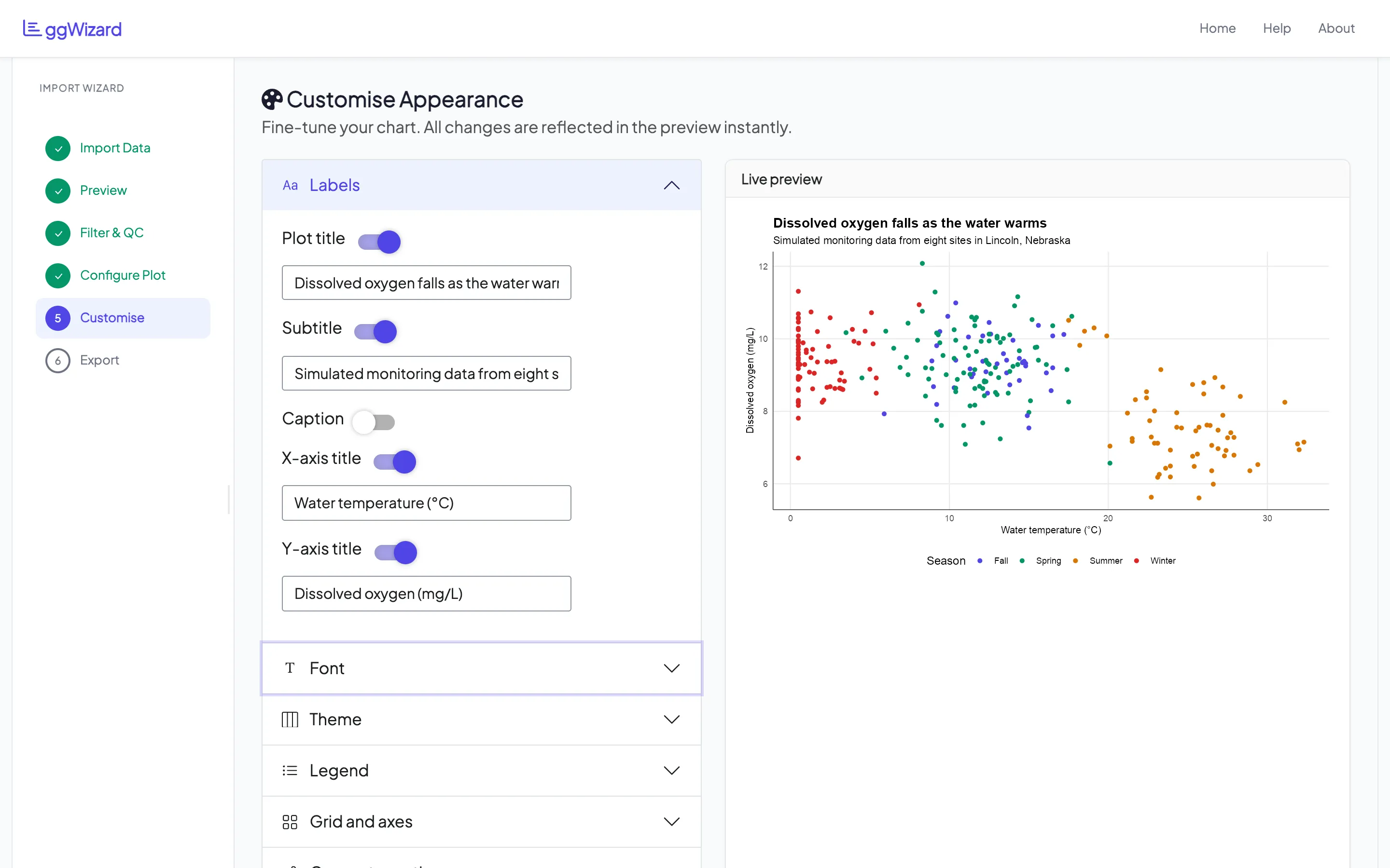
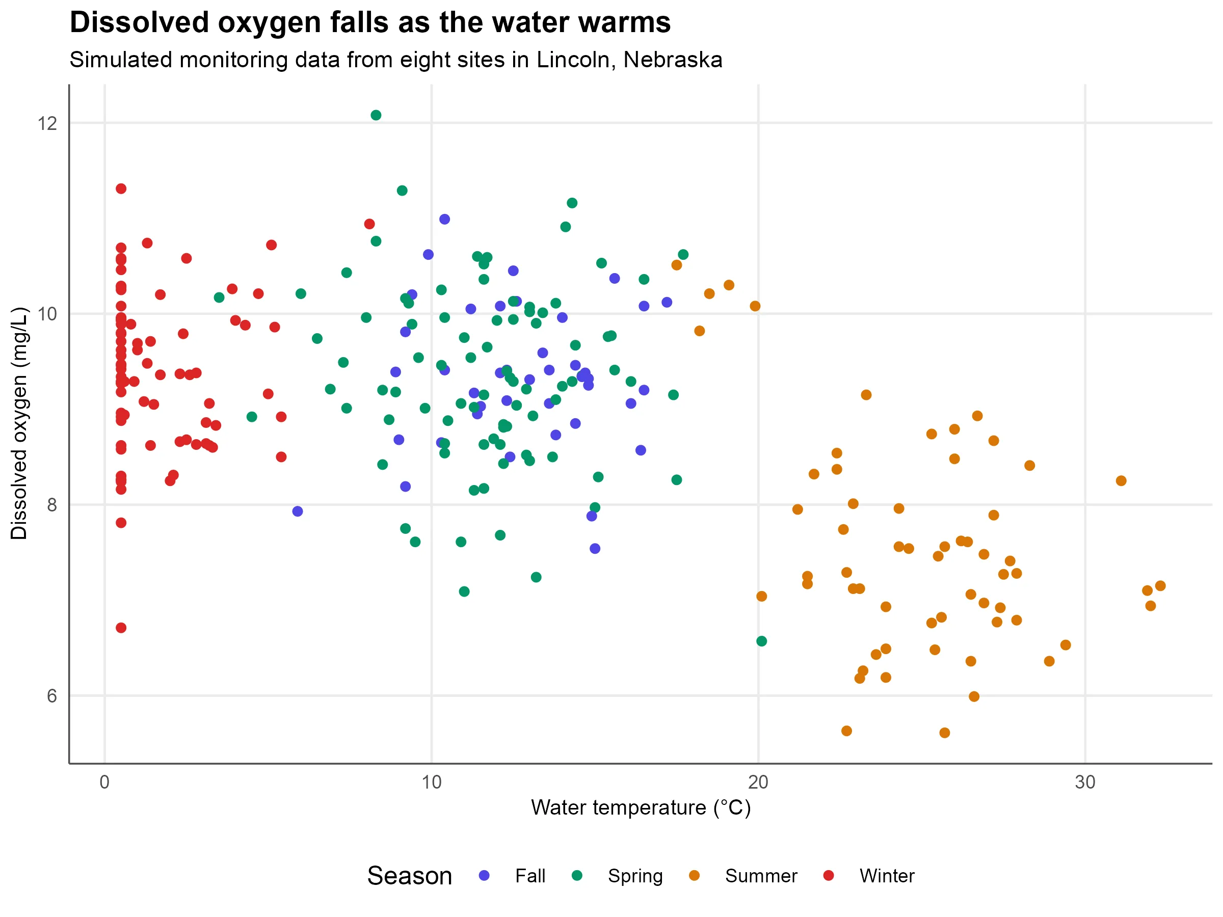
The scatter below is water temperature against dissolved oxygen, coloured by season. Warmer water holds less oxygen. Even the simulated data shows it.
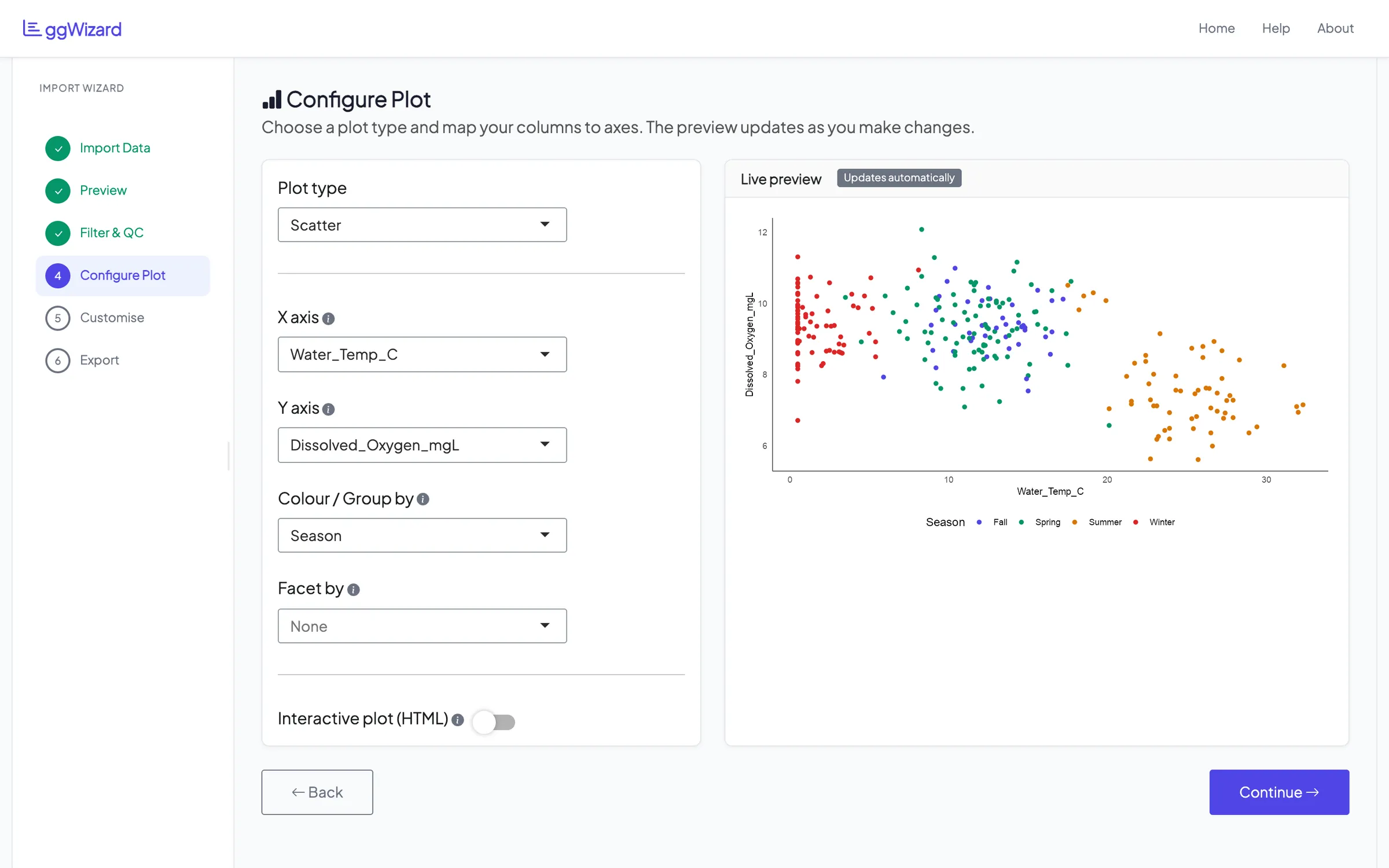
One switch turns the static ggplot2 chart into an interactive plotly one, with hover and zoom. You can save that as an HTML file at the end.
Make it look right
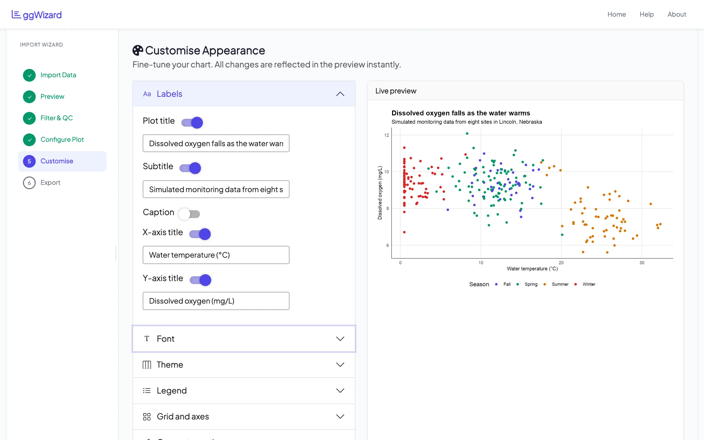
The customise step holds most of the controls, in sections you open as you need them: labels, font, theme, legend, grid and axes. Each label’s text box appears when you switch it on.
Font sizes come as four presets, from small to extra large, that scale every bit of text together. There are also five base themes and palette presets, including Viridis and ColorBrewer. You can switch gridlines and axis lines on and off and set axis ranges, breaks, label angles and margins. Some settings only make sense for one kind of chart, such as the median line and mean marker on a box plot.
Take it with you
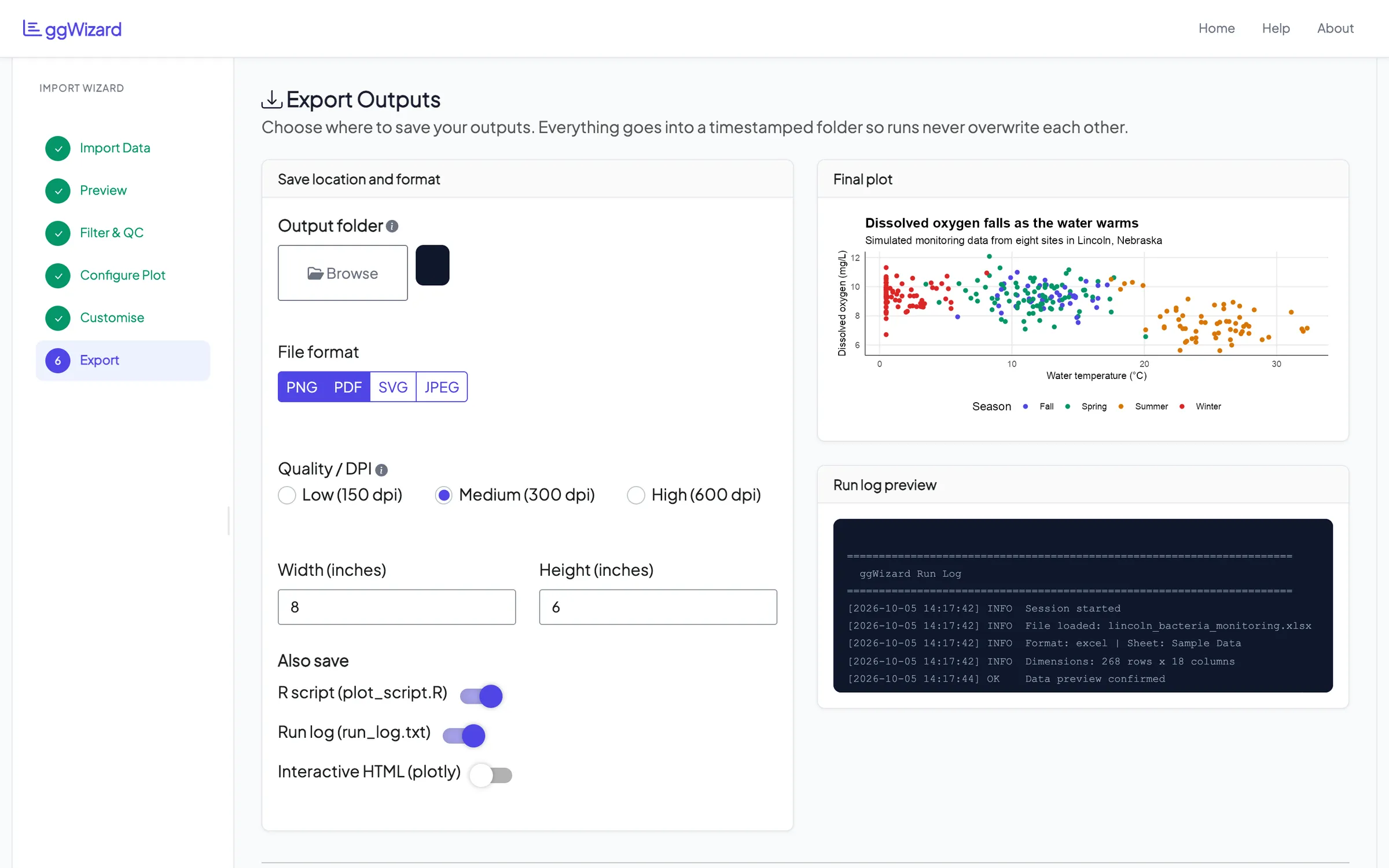
The last step saves the chart as PNG, PDF, SVG or JPEG, at 150, 300 or 600 dpi and whatever size you set. Each save goes into a new timestamped folder, so nothing gets overwritten. You can also download any file on its own without saving anything to disk.
Two extras come with the chart by default, an R script and a run log. The script is plain ggplot2, so you can read exactly how the chart was built. Here’s the main part of the script it wrote for the chart above, trimmed a little:
p <- ggplot(data, aes(x = Water_Temp_C, y = Dissolved_Oxygen_mgL,
                      colour = Season, fill = Season)) +
  geom_point(size = 2.0, shape = 16) +
  theme_minimal(base_size = 12, base_family = "Arial") +
  labs(
    title    = "Dissolved oxygen falls as the water warms",
    subtitle = "Simulated monitoring data from eight sites in Lincoln, Nebraska",
    x        = "Water temperature (°C)",
    y        = "Dissolved oxygen (mg/L)"
  )
The run log records each step with a time: the file and sheet, the size of the data, the chart settings and whether it built.
Where it’s at
ggWizard is version 0.1.0, and I’d call it early. It builds and passes R CMD check on r-universe for Linux and macOS, but it doesn’t have tests of its own yet.
You can install it from my r-universe:
install.packages("ggwizard",
  repos = c("https://ebenogoe.r-universe.dev", "https://cloud.r-project.org"))

library(ggwizard)
run_app()
The app opens in your browser. Click Get Started on the welcome screen and it walks you through the rest.